
Partner Insights
Information to advance your business from industry suppliers

Presented by EquipmentWatch

Presented by Michelin North America
Presented by EquipmentWatch

Presented by Michelin North America


Dealers
Heavy equipment dealers can find everything from industry sales and revenue data to current construction equipment values and more here on Equipment World.


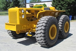
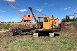
Vintage Equipment
Antique equipment finds

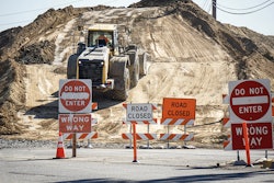
Roadbuilding
Find the most in-depth coverage of road construction projects across the country as well as infrastructure legislation and road-building equipment news here.